Dec. 15, 2005- Jan. 11, 2006 This part of the site is concerned with Latent Class Analysis.
Purpose of this page
I started seriously investigating this area about a week ago due to several factors. In short, I want to find out more about stat methods in social sciences research and will use this page both to report on what I am learning and to give some hints about where source material for this kind of investigation may be accessed in Montreal.
So, this part of the site is something like a blog about learning latent class analysis in Montreal. Although I anticipate having less free time in the future than I currently do, I realize that this is a hefty endeavor and that it should last quite some time.
Some strategy
Although I realize that a lot of software for this kind of model already exists, I plan on writing my own code as I read through the literature and making the code available on this page. Later, I do plan on doing a web search of available software and may add the list to this page.
For the most part, I intend to include enough info about each article or idea that a person with a background similar to mine (MSc Stats) can reproduce my work without having to access the original sources. Still, I guess if a person intends to do original work in this area she will have to go back to the original sources. For example, in Goodman's pub below he spends a lot of important time discussing the very important topic of methods for determining when a model is identifiable. For the moment, I don't plan on writing about this topic. However, if I actually get a chance to analyze some of this type of data, I'll probably write about this topic at that time.
Introductory reading?
One of the first things that one notices when one starts looking at the literature in this field is that Dr. Leo Goodman has made seminal contributions. After doing some reading on the web, I went to the bibliothèque de l'École Polytechnique de Montréal and copied the article Goodman, L. A. (1974). Exploratory latent structure analysis using both identifiable and unidentifiable models. Biometrika, 61, 215-231. I thought that would be a good place to start as the Google entry
leo+goodman+exploratory+latent+structure+analysis+biometrika
returns 158 hits.
To a person who is interested in drawing information from data, the promise of this paper, finding "possible explanations of the observed relationships among a set of m manifest polytomous variables", i.e. discovering meaningful clusters from m-way contingency tables, is likely a very interesting idea.
After spending some hours reading about this topic on the web, I compiled a short list of possible introductory readings. This is shown below.
| What | Where |
|---|---|
| Goodman, L. A. (1974) Exploratory latent structure analysis using both identifiable and unidentifiable models. Biometrika, 61, 215-231 | I've got it in my hands and discuss it below. |
| Goodman, L. A. (1974) The analysis of systems of qualitative variables when some of the variables are unobservable. Part I. A modified latent structure approach. Am. J. Sociol., 79,1179-259. | Long paper. But large type! I've got it from U de M and hope to discuss it in the future, right here. |
| Uebersax JS. (1993) Statistical modeling of expert ratings on medical treatment appropriateness. Journal of the American Statistical Association, 1993, 88, 421-427. | Short paper. I haven't got it yet but may skip to it if the length of previous paper proves daunting. This guy seems to have contributed a lot to this area. His website seems to be full of info as well as being a great portal for further surfing. |
| McCutcheon, Allan L. (1987) Latent class analysis, Sage Publications. | Available at U de M in two libraries, Ed. phys and L.S.H. (which is, I think, the big main library). |
| Jacques A. Hagenaars, Allan L. McCutcheon (2002) Applied latent class analysis, Cambridge University Press. | Copies in Montreal are at McGill and UQAM (according to the interlibrary search utility of the U de M Atrium catalogue). |
Goodman, L. A. (1974). Exploratory latent structure analysis using both identifiable and unidentifiable models.
In studying this paper, I write programs which generate the results of two of the models discussed. I investigate first his model H1, the unrestricted latent class model. Here I describe both the model and Goodman's method for estimating its parameters. This is a model with two latent classes. Then I examine his model H4'', a model with three latent classes. Both of these models are based on the data in the table immediately below.
| Table 1. Observed cross-classification of 216 respondents with respect to whether they tend toward universalistic (1) or particularistic (2) values in four situations of role conflict (A, B, C, D) | ||||
|---|---|---|---|---|
| A | B | C | D | Observed frequency |
| 1 | 1 | 1 | 1 | 42 |
| 1 | 1 | 1 | 2 | 23 |
| 1 | 1 | 2 | 1 | 6 |
| 1 | 1 | 2 | 2 | 25 |
| 1 | 2 | 1 | 1 | 6 |
| 1 | 2 | 1 | 2 | 24 |
| 1 | 2 | 2 | 1 | 7 |
| 1 | 2 | 2 | 2 | 38 |
| 2 | 1 | 1 | 1 | 1 |
| 2 | 1 | 1 | 2 | 4 |
| 2 | 1 | 2 | 1 | 1 |
| 2 | 1 | 2 | 2 | 6 |
| 2 | 2 | 1 | 1 | 2 |
| 2 | 2 | 1 | 2 | 9 |
| 2 | 2 | 2 | 1 | 2 |
| 2 | 2 | 2 | 2 | 20 |
In order to be very sure that I well understand what Goodman is doing in this paper, I write a few R codes that reproduce his results. These are made available and summarized in the table below.
| model-H1.txt contains a function that first writes the data from Table 1 above to an array then uses the algorithm described in the link previously given above to estimate the parameters of model H1. |
| model-H4-db-ABC-only.txt contains a function that first projects the data from Table 1 above onto an array in only the variables A, B, and C and estimates the parameters of a 2-latent class model for this compressed data set. This is the first stage of estimating the parameters in the model H''4. |
| model-H4-db-BCD-only.txt contains a function that first projects the data from Table 1 above onto an array in only the variables B, C, and D and estimates the parameters of a 2-latent class model for this compressed data set. This is the second stage of estimating the parameters in the model H''4. |
| model-H4-db-combine-estimates.txt contains code that compares the estimates from each of the 2-latent class models produced by the codes listed immediately above and produces one set of starting values to be used in the final stage. |
| model-H4-db-final.txt contains a function that accepts some starting values for a restricted three-latent class model of the data from Table 1 above and provides finished estimates for such a model. This is the fourth and final stage of estimating the parameters in the model H''4. |
| Goodman-Biometrika-61-1974.txt is a file containing code which calls each of the functions above and uses their output to create the graphics below. |
Note that graphical results similar to those shown below may be generated by any reader with a suitably configured installation of R who starts an R session and enters "source("http://stat-help.net/Goodman-Biometrika-61-1974.txt")".
Model H1
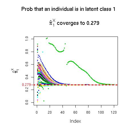
The code in model-H1.txt writes an R function that creates the 4-way contingency table, calculates the parameters of the model and the likelihood ratio chi-squared from a variety of starting vectors and returns all of this information. Note that, as Goodman says, this model is identifiable. Also, there seems to be no problem of local minima here; it seems that, regardless of the starting configuration, the program always returns the set of estimates of πX as { 0.279, 0.721}. However, which of these is returned as π1X is completely arbitrary. Therefore, I added some lines to my code that specify π1X as the smaller of these two estimates, and that reorder the other estimates returned accordingly. After this, as seen in the graphic below, the correct estimate of π1X is always returned, regardless of the starting value.
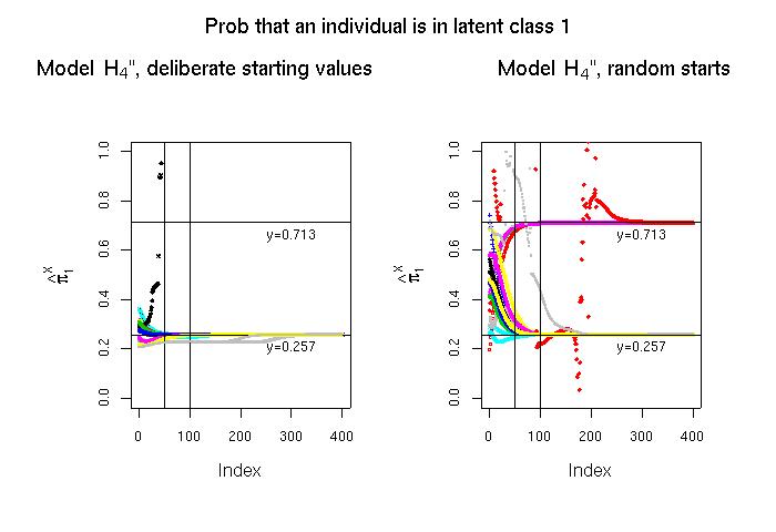
Model H4''
The model Model H4'' is a three latent class model. In this model, the following pairs of probs are the same:
| π11\bar{A}X and π12\bar{A}X |
| π11\bar{B}X and π12\bar{B}X |
| π12\bar{C}X and π13\bar{C}X |
| π12\bar{D}X and π13\bar{D}X. |
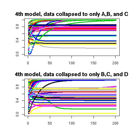
The codes in model-H4-db-ABC-only.txt and model-H4-db-BCD-only.txt both estimate parameters of 2-class models. The top output below shows the estimate of either π1X+π2X or π3X resulting from different starting values. As one may surmise from looking at this output, there are many locally stable sets of estimates here. The bottom graph shows estimates of either π1X or π2X+π3X. Again, there appears to be a plethora of local minima. In both cases, our strategy is simply to draw a big enough sample that something close to the set of estimates globally minimizing the likelihood ratio chi-square will probably be found (we blindly choose a sample of size 60) for each of the two cases. The correct starting values are then discovered by comparing the two sets of estimates. Further details are found here.
Once we have compared the returned values from the 2-class models to arrive at a set of starting values for the 3-class model, we can determine the final estimates for the 3-class model. This is what we do in the below left panel. There we actually go 16 times through the whole process of calling model-H4-db-ABC-only.txt and model-H4-db-BCD-only.txt, determining sets of starting values, and letting the final stage converge. Although it is not the case in the sample drawn here, this process may sometimes lead to the locally valid estimate of π1X=0.713 rather than to the globally valid estimate of π1X=0.257. Therefore, one could simply skip the generation of deliberate starting values (the calls to model-H4-db-ABC-only.txt and model-H4-db-BCD-only.txt), start from random values and let the algorithm for the 3-class model converge, then look for the global minimum likelihood ratio chi-square of 0.9209. This is what I have done in the below right panel.